Analyzing the Performance of NUCAPS Gridded Forecast Parameters and GLM Comparison Between Satellites

 Scattered strong to severe thunderstorms were popping up along the eastern ND and MN border today. However, these storms were struggling to become severe at times with a majority of the cells pulsing up and down. A NUCAPS pass around 19z provided gridded satellite observations and forecasts for the area to compare with SPC’s mesoanalysis page. The gridded NUCAPS at 19z shows CAPE (Image 1) values ranging from 500-1500 J/kg in the area mentioned above with little to no CIN (Image 2) present based on the gridded NUCAPS data. Image 3 below shows the SPC 19z CAPE/CIN data along with the forecast over the next 6 hours (through 01z). When comparing the 19z SPC mesoanalysis to the gridded NUCAPS, there was not much difference between the two with both showing higher CAPE values further south into Nebraska and Kansas. The gridded NUCAPS for CIN seems a bit erroneous with really no signature for -50 or less of CIN, which is present in the SPC mesoanalysis. This is likely due to the lack of detailed boundary layer features with NUCAPS and the fact that it may likely wipe such smaller inversions.

Image 1 shows the 19z gridded NUCAPS for CAPE.

Image 2 shows the 19z gridded NUCAPS for CIN.

Image 3 shows a loop of the MLCAPE/MLCIN forecast values for 6 hours (through 01z) from SPC’s mesoanalysis page.

Looking into the forecasted parameters from NUCAPS, there is a much higher bias in the CAPE values. However, they did a great job at pinpointing an area of higher instability to watch for storms to potentially become more severe with time. The overall CIN forecast looked as if it may start to increase further west near Grand Forks later in the evening, but in central MN where the corridor of CAPE values were higher remained uncapped. As time progressed through the afternoon a few storms did start to intensify and become severe across north central MN with a few severe wind reports. A few lingering surface boundaries were present, along with a weak shortwave at 500mb helped to enhance the storms a bit. I do feel the NUCAPS forecast values for CAPE were a bit too high in comparison to the actual environment and should definitely be compared to model data.

Image 4 is a loop of the 19z gridded NUCAPS forecast of computed CAPE over the next 6 hours (through 01z).

Image 4 is a loop of the 19z gridded NUCAPS forecast of computed CIN over the next 6 hours (through 01z).

Lastly, the location of storms yesterday provided the chance to compare the GOES-16 and GOES-17 GLM products with one another. However, image 5 shows the extent of the two satellites and GOES-17 was right on the edge of where storms were across the Upper Midwest. As you get further away from the satellite and towards the edge of its coverage, you can start to notice more of a tilt in the gridded data. This may cause some erroneous data as seen in comparison with GOES-16. Comparing the GOES-16 data (Image 6) with the GOES-17 data (Image 7), there is a better display of the minimum flash area and lightning sizes with the GOES-16. You can see GOES-16 shows more of a mixture of shorter and longer flashes (purple and yellow colors), while GOES-17 sees strong shorter flashes (yellow colors). Also, the further away the satellite is to the storms the more likely the flash extent density may be less accurate. This is likely due to the storms being on the edge of the satellite’s reach. Therefore it is important to check out both satellites when possible, but take into account where the storms are in respect to the satellites coverage.

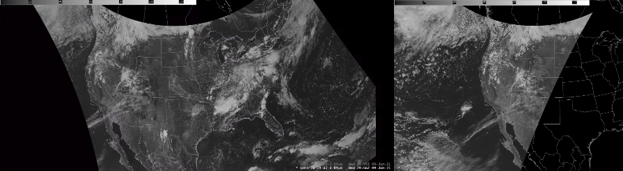
Image 5 shows the areal coverage of GOES-16 (left) and GOES-17 (right).

Image 6 shows GLM through GOES-16 with the local radar (top left), minimum flash area (top right), flash extent density (bottom left) and optical energy (bottom right).

Image 7 shows GLM through GOES-17 with the local radar (top left), minimum flash area (top right), flash extent density (bottom left) and optical energy (bottom right).

Here are a few more supplemental images of the GLM GOES-16 satellite versus the GOES-17 with similar concerns as mentioned above.

Image 8 shows GLM through GOES-16 with the local radar (top left), minimum flash area (top right), flash extent density (bottom left) and optical energy (bottom right).

Image 9 shows GLM through GOES-17 with the local radar (top left), minimum flash area (top right), flash extent density (bottom left) and optical energy (bottom right).

– Harry Potter

Using Optical Wind Flow

 Illustrating how this product can be used during the convective season for different wind fields from the boundary layer, up to the jet stream level.

Mid To Upper Level Winds – Using it for speed, direction and divergence aloft.

All Winds – Can be used for Low Level Jet and boundaries.

– wxboy65

Using NUCAPS

 Are the modified soundings realistic above the mixing layer?

Modified – Note the unusual dry layer around 500 MB.

Unmodified – Note the dry layer around 500 MB isn’t there.

More visually attractive on the SHARP.py vs. NSHARP in Awips.

Comparing soundings across the Northern Plains, and Upper Midwest. (Eastern Mt to the Arrowhead of Mn)

– wxboy65

Analysis of a Line of Storm Moving Across Northeastern LA into Western MS

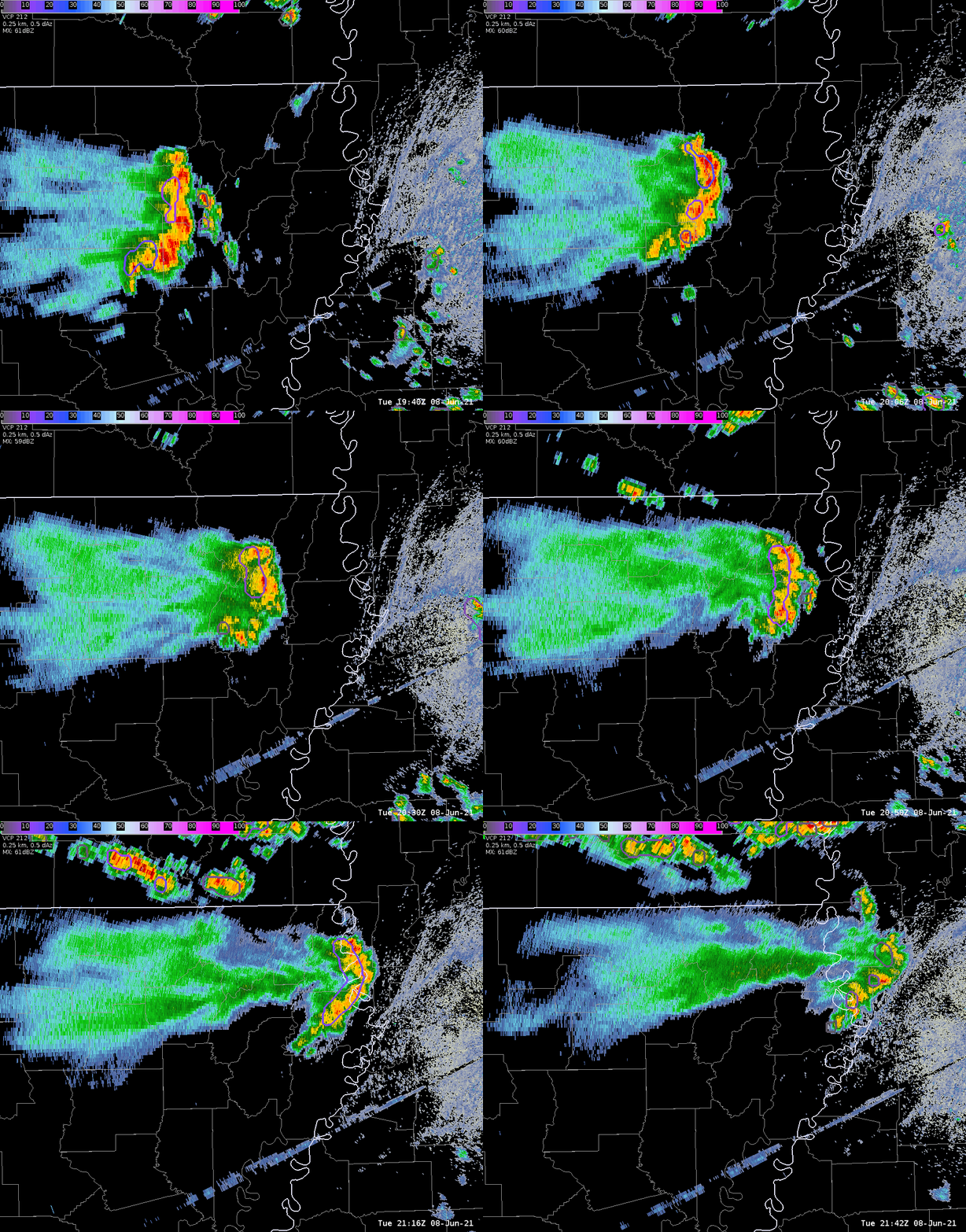
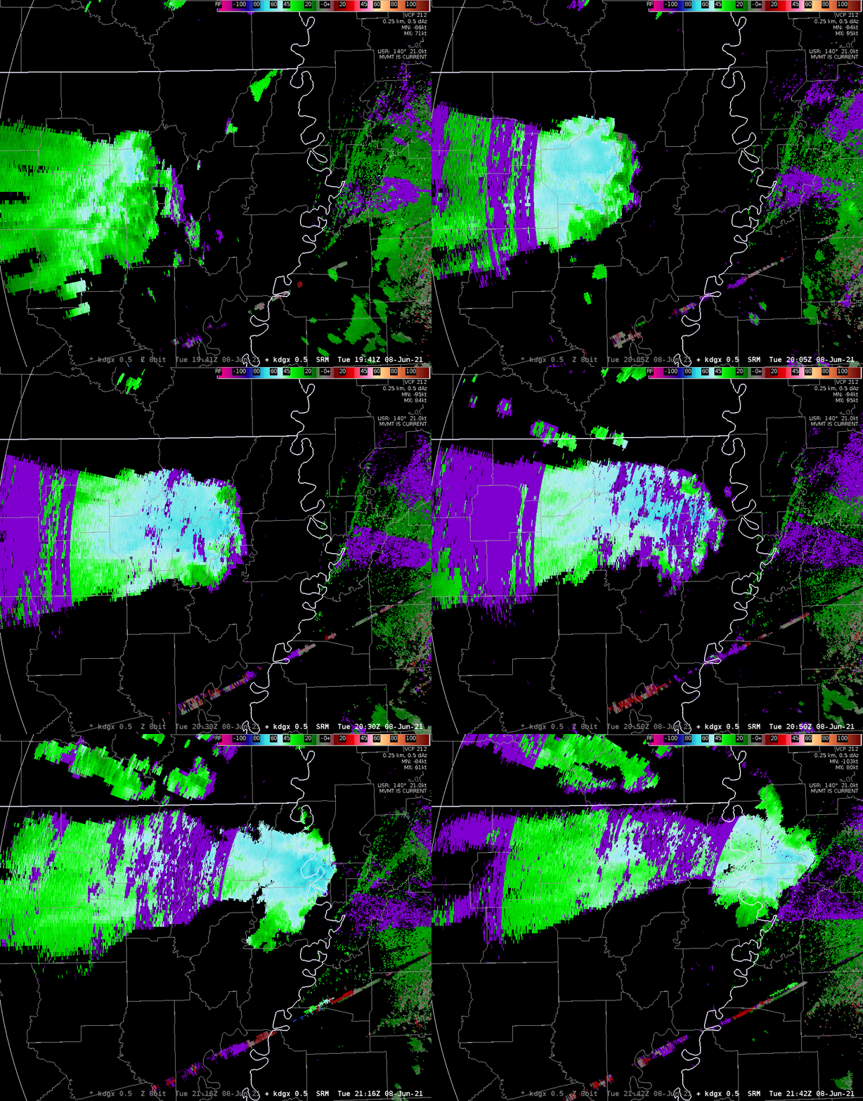
 Today we focused on the slight risk across the southeast, specifically WFO Jackson, MS. During the afternoon hours, a small linear complex was coming across northern LA towards Jackson’s CWA. Right before the CWA line, there was a wind report of snapped tree limbs of 3” diameter from Monroe Airport. There was also a measured gust from the airport of 41 mph. The velocity on radar had ~60 knot outbound winds at around 14,000 – 15,000 feet, which easily could have produced a few severe gusts to the surface. The gifs below show the linear line of storms and the associated velocity as the system moved over Monroe Airport in northeast LA with the wind report at 1952z and then continued to enter western MS.

Image 1 shows a loop of radar reflectivity with prob severe overlaid and Image 2 shows the velocity associated with the radar loop.

In this situation, prob severe was not doing as good of a job on picking up on these “stronger” winds. Image 3 below shows the time of the wind damage report and 41 mph gust at the airport in northeast LA, but prob severe and prob wind are both only picking up about 20% probability of this potential. Almost two hours later, the line of storms are a bit weaker on reflectivity but just as strong or even stronger on velocity. Note, the storms were also closer to the radar at Image 4, so the stronger outbound velocities were closer to the surface. So this led to wondering is prob severe a good indicator for straight line winds?

Image 3 shows the prob severe time series at the time of the damaging wind report at Monroe Airport in northeast LA.

Image 4 again shows a prob severe time series for the same line of storms about two hours later and approaching the western MS border.

Prob severe utilizes azimuthal shear which as seen in the Images 3 and 4 below are not present with solely outbound velocities and little to no inbound present. This is common for straight line wind scenarios, but not super helpful in terms of how prob wind is calculated. Also, the prob severe is an object oriented product that utilizes reflectivity for these objects. In this scenario, the reflectivity definitely began to weaken but velocity did not. The toughest part was the prob severe began to decrease over the two hour time span shown above, but yet several damaging wind reports of roofs blown off and trees/power lines down led me to believe the probability of prob wind should have remained constant or increased over time.

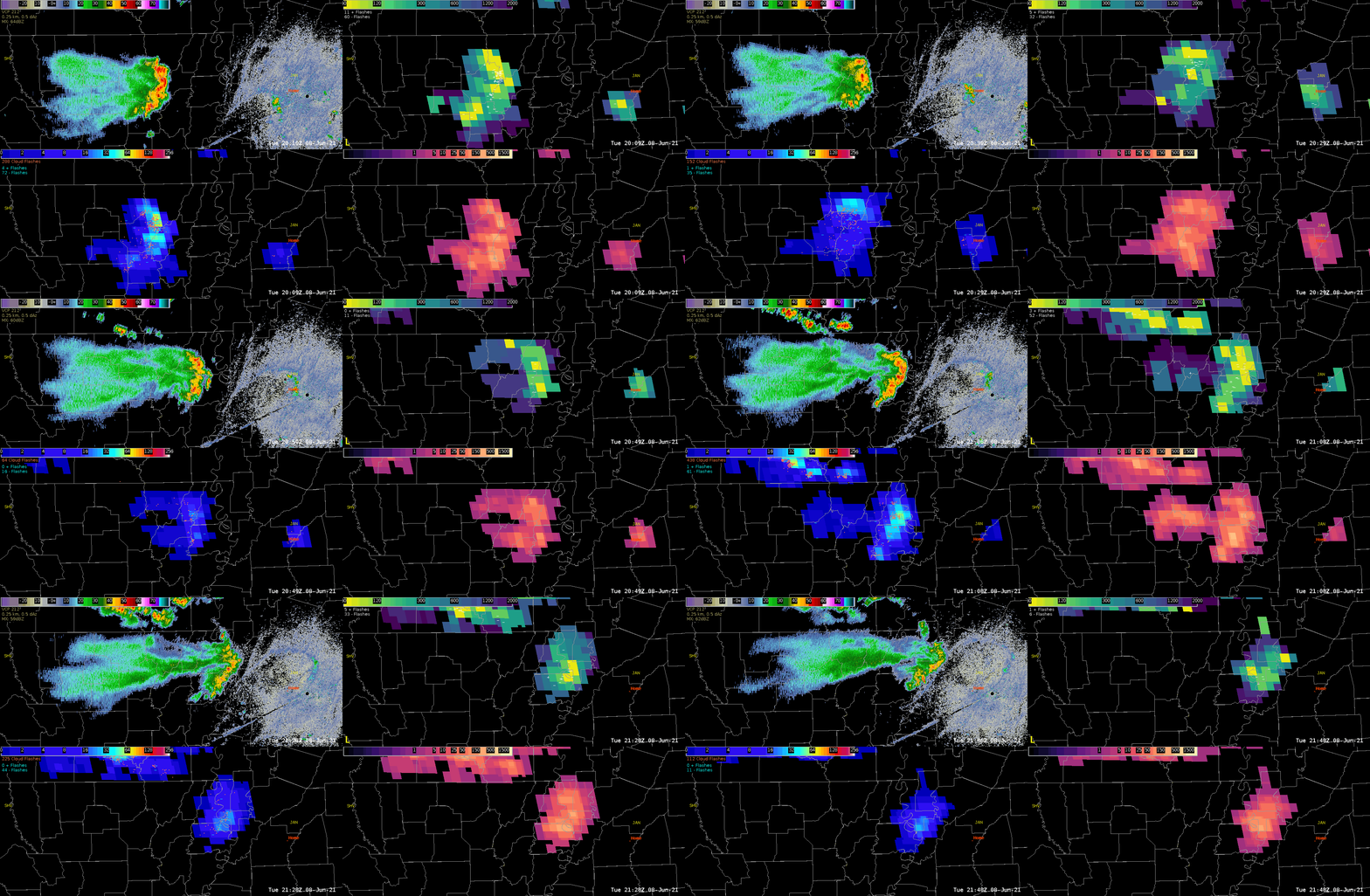
While investigating the prob severe I also took a look into the lightning characteristics within the line as you can see in the GIF below (Image 5) that there is the formation of some trailing stratiform on reflectivity. A still image was taken (Image 6) to show how the lightning began to extend westward into the light stratiform. The flash area (top right of the four panel) shows the darker purple color extending westward, which indicates the storm mode is more of that light stratiform rain with longer flashes extending through it rather than the intense small flashes within the leading line. This can be helpful in time when you may have a DSS event and the main line has passed through, but lightning is still present in the trailing light rain. Pairing the ground networks with the GLM extent and area allows a forecaster to give DSS on the latest CG stroke within the large area.

Image 5 shows a four panel with reflectivity (top left), GLM flash area (top right), GLM flash extent (bottom left) and GLM optical energy (bottom right). The ground networks have been added to the flash area with CG strokes and then over the flash extent with polarity and cloud flashes.

Image 6 shows the same four panel layout as described in image 5, but as a still image. This shows a great use of GLM for examining storm mode and flash extent, along with DSS uses of CG strokes within the large westward expanding extent of flashes behind the main line of storms.

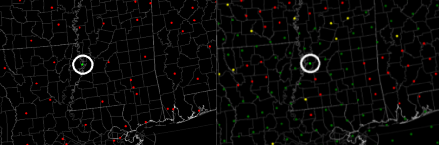
Lastly, there was a NUCAPS CONUS NOAA-20 satellite pass at around 19z, which was well before the line of storms made it to the western Jackson CWA line. No special radiosonde launches were made by local offices, so the next best observational guess of the atmospheric profile would be from satellite. Model soundings were also available to compare at the time. A RAP sounding at 19z was taken just east of the western MS border (see Image 7 below for location of this sounding) and a very nearby NUCAPS sounding was also retrieved for comparison (see Image 8 below for location of this sounding).

Image 7 (left) shows the location of the retrieved 19z RAP sounding (circled in white) and Image 8 (right) shows the location of the retrieved 19z NUCAPS sounding (circled in white).

The soundings (Image 9 and 10 below) looked fairly similar between the model and satellite profiles; however, there were several major differences that played a key role in changing the instability parameters. The NUCAPS sounding was still slightly too low of a surface temperature with 86 deg F versus the RAP’s 89 deg F. Surface observations from 19z at that location showed a temperature of  around 91 deg F. Also, the surface dewpoint was far too low on the NUCAPS profile at the surface as it was 5 degrees below the current observation at 19z. Meanwhile, the RAP was only one degree lower than the current surface dewpoint. These subtle differences caused significant variations in the CAPE values.

Image 9 shows the 19z RAP sounding through sharppy.

Image 10 shows the 19z NUCAPS sounding from sharppy.

After realizing the NUCAPS profile was not accurately depicting the surface temperature/dewpoint, I decided to see what the modified sounding might look like through NSHARP. Image 11 below shows the modified NUCAPS sounding through NSHARP with a much cooler surface temperature of near 80 deg F. This was almost 10 deg below the actual surface temperatures and 6 deg below the original NUCAPS profile. The boundary layer was not representative due to this drastic difference and therefore the modified sounding had to be thrown out of the comparison.

Image 11 shows the modified 19z NUCAPS sounding shown through NSHARP.

Lastly, with knowing the line of storms were headed into the area of interest I decided to see how the forecast products were looking. Unfortunately, I did not get to save the images off in time as the forecast images disappear from AWIPS when the next pass occurs. So I was left with the web-browser version which is only in a gridded format. Unfortunately it is very difficult to depict changes in this format, whereas in AWIPS you can interpolate the image and smooth the results for a more concise display of values. Image 13 shows the comparison of the web-browser gridded format versus the AWIPS smoothed version for the West Coast pass of the NOAA-20 satellite.

Image 13 shows the gridded NUCAPS CAPE forecast for 6 hours in the future from the web-browser (left) and the same exact data and image displayed in AWIPS smoothed (right).

– Harry Potter

Lightning DSS for the Mississippi Pickle Fest

 Our team, as WFO/JAN, chose the setup for the Mississippi Pickle Fest at 1150 Lakeland Drive Jackson, MS as our IDSS location today (Tue, 08 Jun).  Per SPC Outlooks, the Jackson area was on the “edge” of the Marginal Risk Area for severe weather.  As operations began for today, a thundershower was noted to the SW of Jackson, moving NE toward the IDSS location of interest:

KDGX reflectivity at 1926 UTC, with shower SW of Jackson/Pickle Fest. Range rings at 5/10/20 miles.

GLM and NLDN Lightning at 1932 UTC, showing electrical activity in thundershower SW of Jackson, MS.

A modified NUCAPS sounding from near Jackson, MS (which became available later), indicated plenty of instability/CAPE (2000-3500 J kg-1), suggesting that the thundershower would be maintained as it advected toward the Pickle Fest location.  This would be a good time for a “heads-up” to the event venue or EM.  The unmodified NUCAPS sounding (not shown) still suggested sufficient instability aloft for the storm to maintain itself.

The ProbLightning product on the Web, somewhat surprisingly, still showed only ~25% chance of a GLM lightning flash within the next 60 minutes at 2001 UTC, but this had increased to 75% by 2026 UTC:

By 2029 UTC, the electrical activity was nearly overhead:

Interestingly, the NUCAPS forecast CIN was forecast to increase over the next couple of hours (valid 22UTC, below), after the storm passed, but ahead of another, stronger line further upstream (not shown).

Based on this, and the rapid collapse of electrical activity within the shower around 2110 UTC, a reasonably confident “all-clear” could have been given to the venue at that time…or at least until the upstream line approaches in a couple of hours, assuming it holds together.

– ProfessorFrink

Optical Flow Winds On Tuesday - 2105 - 2202 Z

 Today operations were centered over Bismarck, ND, where a large storm complex was in progress much of the day.  The storms developed near a warm front, and benefitted from an approaching short wave trough as well as orographic lift and differential heating.  You can see the extent of the anvils from storms centered over southern ND and northern SD.  This complex dominated the local environment and seemed to take advantage of most of the local instability.

The new optical flow winds tool uses 1-minute imagery from GOES-16/17 ABI imagery to provide high resolution wind estimates at 2-km resolution using an optical flow technique.  You can plot the winds in different layers, from 1000-800mb up to 100-50mb.  As you can see, it is mainly the higher level winds that were plotted above the anvil plumes, and show the divergence at the higher levels of the storm.  

Optical flow winds over storms in southern ND on the afternoon of June 8, 2021.

Taking a look at the SPC mesoanalysis at 300mb for this time, you can see the speeds and directions roughly match the 400-200mb winds plotted on the optical flow plots.

SPC 300mb analysis including heights, divergence, and winds at 2100Z.

Winds closer to the surface did not plot as much, mainly owing to the dense cloud cover the satellite was seeing.  After some discussion, surface plots were added to the 1000-800mb layer, which helped to orient forecasters.  Forecasters still need to mentally adjust the satellite imagery which was overlaid for parallax.

Optical winds with station plots added.

I think the optical wind flow could be useful to investigate storm strength and maintenance.  It could be helpful in both warning operations and for IDSS purposes.  The storm complex in question lasted for at least 12 hours, and produced wind damage, large hail, and torrential rains leading to flash flooding. 

– Dana Scully

Using GLM

 Using the minimum flash area to show where the smaller lightning strikes occur but is associated with stronger updraft with cells building faster (Yellow) to generate lightning. Larger lightning strikes occur in the stratiform area of the precipitation field where charge building is slower (Purple). This is also a good way to indicate convective mode as the system translates from individual (SuperCell) to a linear mode.

(Upper Left – ProgSvr/Ref), (Upper Right – Flash Extent Density), (Lower Left – Optical Energy), (Lower Right – Minimum Flash Area) Note the area of enhancement behind the main convective line. This is stratiform lightning strikes where the charges are slower to build vs. the convective linear line, and individual cells out in front of the storm.

Note the differences from the previous image as the Optical/FED and Minimum Flash Area has less flashes. This is due to the building of the charges.

A four panel of GR2 where reflectivity (Upper Left), and ZDR (Lower Right) depict linear striations (above melting level – 30 dBz) to show the build-up of charges in the stratiform area of the storm. A good way to use it is for IDSS and the likeability of lightning strikes developing.

Using NUCAPS (Modified vs. Unmodified). Why the CAP at mid-levels noted in Arkansas? Is this reasonable or an artifact of the program that isn’t real.

Unmodified

Modified

– wxboy65

Utilizing NUCAPS Profiles to Analyze the Pre-Convective Environment Across West Texas

 WFO Amarillo launched a 19z special sounding today in support of potential severe storms later in the evening. Meanwhile, NOAA-20 passed over WFO Amarillo at 1935z, merely 30 minutes after the observed sounding release but likely about an hour before the full observed profile was complete.

An SPC marginal risk was over west Texas (see below) for the 20z issuance with the main threats being large hail and damaging wind gusts. The 12z observed sounding from Amarillo shows a pronounced low level capping inversion with a convective temperature of around 86 degrees F. Overall, the wind profile is weak with little to no shear but just enough to support a few strong to severe storms. Mixed layer CAPE is around 1000 J/kg, but the downdraft CAPE is closer to 1200 and supports the potential for some strong to damaging wind gusts with collapsing storms and/or areas conducive to strong downward motion.

Image A: 12z Observed Sounding from AMA on June 7, 2021.

Sharppy was then utilized to compare the observed 19z sounding from Amarillo to the closest NUCAPS sounding to the office’s location. Image B contains the values for the observed sounding with the purple representing the sharppy NUCAPS sounding. Image C contains the values for the sharppy NUCAPS with the observed sounding in purple. One of the biggest differences between the soundings that plays a key role in the instability parameters is the surface temperatures. The observed sounding recorded a surface temperature of 83 degrees F, which the sharppy NUCAPS sounding recorded a surface temperature of 89 degrees F. That difference of 6 degrees fully breaks the capping inversion on the sharppy NUCAPS sounding, but the observed sounding still appears to be a few degrees shy of breaking the 750mb cap. The values such as MLCAPE are drastically different with the observed sounding showing around 1500 J/kg, while the sharppy NUCAPS sounding shows ~2500 J/kg. The observed sounding does show an increase since the 12z launch of DCAPE now around 1600 J/kg, but the sharppy NUCAPS does not relay this same increase and instead remains near 1200 J/kg.

Image B: 19z observed sounding (colored) compared to the 1935z sharppy NUCAPS sounding (purple). The values represent the observed sounding.

Image C: 1935z sharppy NUCAPS sounding (colored) compared to the 19z observed sounding (purple). The values represent the sharppy NUCAPS sounding.

So the biggest fault in the NUCAPS values being off was likely the surface temperatures being too warm. In order to validate this reasoning, the modified NUCAPS sounding for this time and location was utilized. However, since the modified soundings are calculated with NSHARP and not sharppy, the original NUCAPS from both algorithms were compared. Image D shows the NSHARP NUCAPS sounding pulled from the CAVE in awips. This can be compared to Image C, which was the NUCAPS sounding plotted with a different program called sharppy.

Looking at the profile itself, the biggest difference that stands out would be near the surface. As stated before the surface temperature on the sharppy NUCAPS sounding was 89 deg F, while the NSHARP sounding reveals a surface temperature of around 80 deg F. The NSHARP sounding temperature is lower than the observed sounding at 19z, but yet was able to mix out the capping inversion. Knowing that NUCAPS in general is not overly impressive with the boundary layer, there is a chance had there been a 12z pass, that the NUCAPS sounding wouldn’t have had such a strong inversion as the observational sounding at 12z showed. Therefore the surface temperature wouldn’t have needed to be as warm. The remainder of the parameters seem to compare pretty well between the two versions of the NUCAPS profile.

Image D: 1935z NSHARP NUCAPS sounding from CAVE.

Now, what happens if the surface temperature from observations are used to modify the NSHARP NUCAPS profile for better representation of that boundary layer. Image E represents this modified sounding where the surface temperature is now closer to 83 deg F, which is what the 19z observed sounding from the same location measured. Comparing this modified sounding to the observed, there is still the issue of the NUCAPS wiping out the inversion layer at around 750 mb. Warming the temperature was not going to bring the inversion back, so this is something that is more a failure starting with the non-modified NSHAPR NUCAPS profile. MLCAPE is still significantly different, but ignoring the inversion in the observed sounding and looking at a surface based parcel, the two soundings are pretty comparable with around 3500 J/kg of SBCAPE. Downdraft CAPE values did not change with the modified NSHARP NUCAPS sounding and this could allude to the fact that again the NUCAPS profiles lack good boundary layer details and a much smoother profile.

Overall, had Amarillo not done a 12z launch, the NUCAPS profiles were pretty comparable to the observed sounding. The biggest concern would be if the purpose was to find if there still remains a capping inversion in place that may hinder storm development. Spoiler alert, storms did develop as temperatures warmed a bit more through the afternoon and were also just a bit warmer further west along the New Mexico/Texas border. A few severe wind reports occurred with the cluster of storms, along with some small hail and maybe even a few larger hail stones of around a quarter that weren’t reported.

– Harry Potter